.

Correlation Analysis

Correlation

  • Is a measure of association between two quantitative variables.

  • Purpose is to measure the strength and direction of the relationship between two variables.

\[ r_{xy} = \frac{\Sigma_{i=1}^n (x_i - \bar x) (y_i - \bar y)}{\sqrt{\Sigma_{i=1}^n (x_i - \bar x)^2 (y_i - \bar y)^2}} \]

Correlation coefficient interpretation

Correlation coefficient Psychology Politics and economics Medicine
± 1.0 Perfect Perfect Perfect
± 0.9 Strong Very strong Very strong
± 0.8 Strong Very strong Very strong
± 0.7 Strong Very strong Moderate
± 0.6 Moderate Strong Moderate
± 0.5 Moderate Strong Fair
± 0.4 Moderate Strong Fair
± 0.3 Weak Moderate Fair
± 0.2 Weak Weak Poor
± 0.1 Weak Negligible Poor
± 0.0 Zero None None

Correlation

```{r}
# Use the built-in 'mtcars' dataset
data <- mtcars

# Calculate correlation coefficient
correlation <- cor(data$mpg, data$wt)

# Create scatter plot
ggplot(data, aes(x = wt, y = mpg)) +
  geom_point(color = "blue", alpha = 0.7) +
  labs(
    title = "Scatter Plot of Miles Per Gallon vs Car Weight",
    x = "Car Weight (1000 lbs)",
    y = "Miles Per Gallon (MPG)"
  ) +
  annotate("text", 
           x = max(data$wt) * 0.7, 
           y = max(data$mpg) * 0.9, 
           label = paste("Correlation:", round(correlation, 2)),
           size = 6,
           color = "red") +
  theme_minimal()
```

Correlation vs Causation

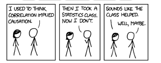
  • two things that goes together may not necessarily mean that there is causation

  • one variable can be strongly related to another, yet not cause it.

  • Correlation does not imply causality.


Correlation

Type Data type When to use
  • Pearson
  • Continuous
  • Normally distributed
  • both variables are continuous and normally distributed and the relationship is linear
  • Spearman
  • Continuous (non-normal)
  • Ordinal
  • when data is ordinal, or the relationship is monotonic but not linear

Pearson correlation

R activity

Test if there is a relationship between mpg and car weight using mtcars dataset.

Step 1: read in data

data(mtcars)
head(mtcars)
                   mpg cyl disp  hp drat    wt  qsec vs am gear carb
Mazda RX4         21.0   6  160 110 3.90 2.620 16.46  0  1    4    4
Mazda RX4 Wag     21.0   6  160 110 3.90 2.875 17.02  0  1    4    4
Datsun 710        22.8   4  108  93 3.85 2.320 18.61  1  1    4    1
Hornet 4 Drive    21.4   6  258 110 3.08 3.215 19.44  1  0    3    1
Hornet Sportabout 18.7   8  360 175 3.15 3.440 17.02  0  0    3    2
Valiant           18.1   6  225 105 2.76 3.460 20.22  1  0    3    1

Step 2: normality test

shapiro.test(mtcars$wt)

    Shapiro-Wilk normality test

data:  mtcars$wt
W = 0.94326, p-value = 0.09265
shapiro.test(mtcars$mpg)

    Shapiro-Wilk normality test

data:  mtcars$mpg
W = 0.94756, p-value = 0.1229

Pearson correlation

Step 3: Create scatterplot

mtcars |> 
  ggplot(aes(wt, mpg)) +
  geom_point(size = 2) +
  theme_minimal(base_size = 12)

Step 4: Perform pearson correlation

cor.test(mtcars$mpg, mtcars$wt, method = "pearson")

    Pearson's product-moment correlation

data:  mtcars$mpg and mtcars$wt
t = -9.559, df = 30, p-value = 1.294e-10
alternative hypothesis: true correlation is not equal to 0
95 percent confidence interval:
 -0.9338264 -0.7440872
sample estimates:
       cor 
-0.8676594 

Spearman correlation

R activity

Test if there is a relationship between mpg and car horse power using mtcars dataset.

Step 1: read in data

data(mtcars)
head(mtcars)
                   mpg cyl disp  hp drat    wt  qsec vs am gear carb
Mazda RX4         21.0   6  160 110 3.90 2.620 16.46  0  1    4    4
Mazda RX4 Wag     21.0   6  160 110 3.90 2.875 17.02  0  1    4    4
Datsun 710        22.8   4  108  93 3.85 2.320 18.61  1  1    4    1
Hornet 4 Drive    21.4   6  258 110 3.08 3.215 19.44  1  0    3    1
Hornet Sportabout 18.7   8  360 175 3.15 3.440 17.02  0  0    3    2
Valiant           18.1   6  225 105 2.76 3.460 20.22  1  0    3    1

Step 2: normality test

shapiro.test(mtcars$hp)

    Shapiro-Wilk normality test

data:  mtcars$hp
W = 0.93342, p-value = 0.04881
shapiro.test(mtcars$mpg)

    Shapiro-Wilk normality test

data:  mtcars$mpg
W = 0.94756, p-value = 0.1229

Spearman correlation

Step 3: Create scatterplot

mtcars |> 
  ggplot(aes(hp, mpg)) +
  geom_point(size = 2) +
  theme_minimal(base_size = 12)

Step 4: Perform spearman correlation

cor.test(mtcars$mpg, mtcars$wt, method = "spearman")

    Spearman's rank correlation rho

data:  mtcars$mpg and mtcars$wt
S = 10292, p-value = 1.488e-11
alternative hypothesis: true rho is not equal to 0
sample estimates:
      rho 
-0.886422 

Check-up quiz

What does correlation analysis aim to determine?

  • The cause-and-effect relationship between two variables.

  • The strength and direction of the linear relationship between two variables

  • The difference in means between two groups.

  • The probability of an event occurring.

Which of the following correlation coefficients indicates the strongest relationship?

  • 0.25

  • -0.70

  • 0.10

  • 0.50

A correlation coefficient of -0.80 suggests:

  • A strong positive relationship.

  • A weak positive relationship.

  • A strong negative relationship

  • No relationship.

What is the range of values for a correlation coefficient?

  • 0 to 1

  • -1 to 1

  • -∞ to ∞

  • 0 to ∞

Which of the following factors can influence the correlation coefficient?

  • Outliers in the data.

  • The units of measurement of the variables.

  • The sample size.

  • All of the above