.

Overview

R objects
R packages
Reading data in R
Basic data wrangling

Illustration adopted from Allison Horst

R Objects

You can consider R objects as saving information
e.g., text, number, matrix, vectro, dataframe
In another words everything in R is an object

R objects

Objects in R are assigned a value using →

a1 <- 10
a1

[1] 10

a2 <- 20
a2

[1] 20

a3 <- c(10, 20, 30)
a3

[1] 10 20 30

a1 + a2

[1] 30

st_name <- "christopher"
st_age <- 23
st_sex <- "male"
student <- c(st_name, st_age, st_sex)

student

[1] "christopher" "23"          "male"

R packages

Collection of functions that load into your working environment.
A package contains code that other R users have prepared for the community.
Installing a package

install.packages("tidyverse")

Loading a package

library(tidyverse)

Importing data

SPSS, Stata, SAS files: haven package
Excel files: readxl package
CSV files: readr package

Importing data into R

SPSS, Stata & SAS using haven package

# loading haven package
library(haven)

# SPSS
read_sav("path/data.sav")

# Stata
read_dta("path/data.dta")

# SAS
read_sas("path/data.sas7bdat")

Importing data into R

Excel files using readxl package

library(readxl)
read_excel("path/dataset.xls")

# A tibble: 150 × 5
   Sepal.Length Sepal.Width Petal.Length Petal.Width Species
          <dbl>       <dbl>        <dbl>       <dbl> <chr>  
 1          5.1         3.5          1.4         0.2 setosa 
 2          4.9         3            1.4         0.2 setosa 
 3          4.7         3.2          1.3         0.2 setosa 
 4          4.6         3.1          1.5         0.2 setosa 
 5          5           3.6          1.4         0.2 setosa 
 6          5.4         3.9          1.7         0.4 setosa 
 7          4.6         3.4          1.4         0.3 setosa 
 8          5           3.4          1.5         0.2 setosa 
 9          4.4         2.9          1.4         0.2 setosa 
10          4.9         3.1          1.5         0.1 setosa 
# ℹ 140 more rows

Importing data into R

CSV files using readr package

install.packages("readr")
library(readr)

# comma separated (CSV) files
read_csv("path/data.csv")

# tab separated files
read_tsv("path/data.tsv")

# general delimited files
read_delim("path/data.delim")

Basic data wrangling with Tidyverse

What is tidyverse?

A collection of R packages designed for data science.

All packages share an underlying philosophy, grammar, and data structure.

Illustration adopted from Allison Horst

Tidy data makes it easier for reproducibility and reuse

Illustration adopted from Allison Horst

Yehey! Tidy Data for the win!

Illustration adopted from Allison Horst

Data wrangling using `dplyr`

Illustration adopted from Allison Horst

`dplyr`

Overview

select() picks variables based on their names
mutate() adds new variables
filter() picks cases based on their values
summarise() reduces multiple values down to a single summary
arrange() change the ordering of the rows

`select()`

data

data
# A tibble: 1,704 × 6
   country     continent  year lifeExp      pop gdpPercap
   <fct>       <fct>     <int>   <dbl>    <int>     <dbl>
 1 Afghanistan Asia       1952    28.8  8425333      779.
 2 Afghanistan Asia       1957    30.3  9240934      821.
 3 Afghanistan Asia       1962    32.0 10267083      853.
 4 Afghanistan Asia       1967    34.0 11537966      836.
 5 Afghanistan Asia       1972    36.1 13079460      740.
 6 Afghanistan Asia       1977    38.4 14880372      786.
 7 Afghanistan Asia       1982    39.9 12881816      978.
 8 Afghanistan Asia       1987    40.8 13867957      852.
 9 Afghanistan Asia       1992    41.7 16317921      649.
10 Afghanistan Asia       1997    41.8 22227415      635.
# ℹ 1,694 more rows

select(data, continent, country, pop)

select(data, continent, country, pop)
# A tibble: 1,704 × 3
   continent country          pop
   <fct>     <fct>          <int>
 1 Asia      Afghanistan  8425333
 2 Asia      Afghanistan  9240934
 3 Asia      Afghanistan 10267083
 4 Asia      Afghanistan 11537966
 5 Asia      Afghanistan 13079460
 6 Asia      Afghanistan 14880372
 7 Asia      Afghanistan 12881816
 8 Asia      Afghanistan 13867957
 9 Asia      Afghanistan 16317921
10 Asia      Afghanistan 22227415
# ℹ 1,694 more rows

`select()`

We can also remove variables with a - (minus)

data

data
# A tibble: 1,704 × 6
   country     continent  year lifeExp      pop gdpPercap
   <fct>       <fct>     <int>   <dbl>    <int>     <dbl>
 1 Afghanistan Asia       1952    28.8  8425333      779.
 2 Afghanistan Asia       1957    30.3  9240934      821.
 3 Afghanistan Asia       1962    32.0 10267083      853.
 4 Afghanistan Asia       1967    34.0 11537966      836.
 5 Afghanistan Asia       1972    36.1 13079460      740.
 6 Afghanistan Asia       1977    38.4 14880372      786.
 7 Afghanistan Asia       1982    39.9 12881816      978.
 8 Afghanistan Asia       1987    40.8 13867957      852.
 9 Afghanistan Asia       1992    41.7 16317921      649.
10 Afghanistan Asia       1997    41.8 22227415      635.
# ℹ 1,694 more rows

select(data, -year, -pop)

select(data, -year, -pop)
# A tibble: 1,704 × 4
   country     continent lifeExp gdpPercap
   <fct>       <fct>       <dbl>     <dbl>
 1 Afghanistan Asia         28.8      779.
 2 Afghanistan Asia         30.3      821.
 3 Afghanistan Asia         32.0      853.
 4 Afghanistan Asia         34.0      836.
 5 Afghanistan Asia         36.1      740.
 6 Afghanistan Asia         38.4      786.
 7 Afghanistan Asia         39.9      978.
 8 Afghanistan Asia         40.8      852.
 9 Afghanistan Asia         41.7      649.
10 Afghanistan Asia         41.8      635.
# ℹ 1,694 more rows

`select()`

Selection helpers

These selection helpers match variables according to a given pattern.

starts_with() starts with a prefix
ends_with() ends with a suffix
contains() contains a literal string
matches() matches regular expression

`filter()`

data

data
# A tibble: 1,704 × 6
   country     continent  year lifeExp      pop gdpPercap
   <fct>       <fct>     <int>   <dbl>    <int>     <dbl>
 1 Afghanistan Asia       1952    28.8  8425333      779.
 2 Afghanistan Asia       1957    30.3  9240934      821.
 3 Afghanistan Asia       1962    32.0 10267083      853.
 4 Afghanistan Asia       1967    34.0 11537966      836.
 5 Afghanistan Asia       1972    36.1 13079460      740.
 6 Afghanistan Asia       1977    38.4 14880372      786.
 7 Afghanistan Asia       1982    39.9 12881816      978.
 8 Afghanistan Asia       1987    40.8 13867957      852.
 9 Afghanistan Asia       1992    41.7 16317921      649.
10 Afghanistan Asia       1997    41.8 22227415      635.
# ℹ 1,694 more rows

filter(data, country == "Philippines")

filter(data, country == "Philippines")
# A tibble: 12 × 6
   country     continent  year lifeExp      pop gdpPercap
   <fct>       <fct>     <int>   <dbl>    <int>     <dbl>
 1 Philippines Asia       1952    47.8 22438691     1273.
 2 Philippines Asia       1957    51.3 26072194     1548.
 3 Philippines Asia       1962    54.8 30325264     1650.
 4 Philippines Asia       1967    56.4 35356600     1814.
 5 Philippines Asia       1972    58.1 40850141     1989.
 6 Philippines Asia       1977    60.1 46850962     2373.
 7 Philippines Asia       1982    62.1 53456774     2603.
 8 Philippines Asia       1987    64.2 60017788     2190.
 9 Philippines Asia       1992    66.5 67185766     2279.
10 Philippines Asia       1997    68.6 75012988     2537.
11 Philippines Asia       2002    70.3 82995088     2651.
12 Philippines Asia       2007    71.7 91077287     3190.

`mutate()`

The mutate function will take a statement similar to this:

variable_name = do_some_calculation
variable_name will be attached at the end of the dataset.

`mutate()`

Let’s calculate the gdp

data

data
# A tibble: 1,704 × 6
   country     continent  year lifeExp      pop gdpPercap
   <fct>       <fct>     <int>   <dbl>    <int>     <dbl>
 1 Afghanistan Asia       1952    28.8  8425333      779.
 2 Afghanistan Asia       1957    30.3  9240934      821.
 3 Afghanistan Asia       1962    32.0 10267083      853.
 4 Afghanistan Asia       1967    34.0 11537966      836.
 5 Afghanistan Asia       1972    36.1 13079460      740.
 6 Afghanistan Asia       1977    38.4 14880372      786.
 7 Afghanistan Asia       1982    39.9 12881816      978.
 8 Afghanistan Asia       1987    40.8 13867957      852.
 9 Afghanistan Asia       1992    41.7 16317921      649.
10 Afghanistan Asia       1997    41.8 22227415      635.
# ℹ 1,694 more rows

mutate(data, GDP = gdpPercap * pop)

mutate(data, GDP = gdpPercap * pop)
# A tibble: 1,704 × 7
   country     continent  year lifeExp      pop gdpPercap          GDP
   <fct>       <fct>     <int>   <dbl>    <int>     <dbl>        <dbl>
 1 Afghanistan Asia       1952    28.8  8425333      779.  6567086330.
 2 Afghanistan Asia       1957    30.3  9240934      821.  7585448670.
 3 Afghanistan Asia       1962    32.0 10267083      853.  8758855797.
 4 Afghanistan Asia       1967    34.0 11537966      836.  9648014150.
 5 Afghanistan Asia       1972    36.1 13079460      740.  9678553274.
 6 Afghanistan Asia       1977    38.4 14880372      786. 11697659231.
 7 Afghanistan Asia       1982    39.9 12881816      978. 12598563401.
 8 Afghanistan Asia       1987    40.8 13867957      852. 11820990309.
 9 Afghanistan Asia       1992    41.7 16317921      649. 10595901589.
10 Afghanistan Asia       1997    41.8 22227415      635. 14121995875.
# ℹ 1,694 more rows

`rename()`

Changes the variable name while keeping all else intact.

new_variable_name = old_variable_name

data

data
# A tibble: 1,704 × 6
   country     continent  year lifeExp      pop gdpPercap
   <fct>       <fct>     <int>   <dbl>    <int>     <dbl>
 1 Afghanistan Asia       1952    28.8  8425333      779.
 2 Afghanistan Asia       1957    30.3  9240934      821.
 3 Afghanistan Asia       1962    32.0 10267083      853.
 4 Afghanistan Asia       1967    34.0 11537966      836.
 5 Afghanistan Asia       1972    36.1 13079460      740.
 6 Afghanistan Asia       1977    38.4 14880372      786.
 7 Afghanistan Asia       1982    39.9 12881816      978.
 8 Afghanistan Asia       1987    40.8 13867957      852.
 9 Afghanistan Asia       1992    41.7 16317921      649.
10 Afghanistan Asia       1997    41.8 22227415      635.
# ℹ 1,694 more rows

rename(data, population = pop)

rename(data, population = pop)
# A tibble: 1,704 × 6
   country     continent  year lifeExp population gdpPercap
   <fct>       <fct>     <int>   <dbl>      <int>     <dbl>
 1 Afghanistan Asia       1952    28.8    8425333      779.
 2 Afghanistan Asia       1957    30.3    9240934      821.
 3 Afghanistan Asia       1962    32.0   10267083      853.
 4 Afghanistan Asia       1967    34.0   11537966      836.
 5 Afghanistan Asia       1972    36.1   13079460      740.
 6 Afghanistan Asia       1977    38.4   14880372      786.
 7 Afghanistan Asia       1982    39.9   12881816      978.
 8 Afghanistan Asia       1987    40.8   13867957      852.
 9 Afghanistan Asia       1992    41.7   16317921      649.
10 Afghanistan Asia       1997    41.8   22227415      635.
# ℹ 1,694 more rows

`arrange()`

You can order data by variable to show the highest or lowest values first.

consider lifeExp default is lowest first

data

data
# A tibble: 1,704 × 6
   country     continent  year lifeExp      pop gdpPercap
   <fct>       <fct>     <int>   <dbl>    <int>     <dbl>
 1 Afghanistan Asia       1952    28.8  8425333      779.
 2 Afghanistan Asia       1957    30.3  9240934      821.
 3 Afghanistan Asia       1962    32.0 10267083      853.
 4 Afghanistan Asia       1967    34.0 11537966      836.
 5 Afghanistan Asia       1972    36.1 13079460      740.
 6 Afghanistan Asia       1977    38.4 14880372      786.
 7 Afghanistan Asia       1982    39.9 12881816      978.
 8 Afghanistan Asia       1987    40.8 13867957      852.
 9 Afghanistan Asia       1992    41.7 16317921      649.
10 Afghanistan Asia       1997    41.8 22227415      635.
# ℹ 1,694 more rows

desc() sort lifeExp from highest to lowest

arrange(data, desc(lifeExp))

arrange(data, desc(lifeExp))
# A tibble: 1,704 × 6
   country          continent  year lifeExp       pop gdpPercap
   <fct>            <fct>     <int>   <dbl>     <int>     <dbl>
 1 Japan            Asia       2007    82.6 127467972    31656.
 2 Hong Kong, China Asia       2007    82.2   6980412    39725.
 3 Japan            Asia       2002    82   127065841    28605.
 4 Iceland          Europe     2007    81.8    301931    36181.
 5 Switzerland      Europe     2007    81.7   7554661    37506.
 6 Hong Kong, China Asia       2002    81.5   6762476    30209.
 7 Australia        Oceania    2007    81.2  20434176    34435.
 8 Spain            Europe     2007    80.9  40448191    28821.
 9 Sweden           Europe     2007    80.9   9031088    33860.
10 Israel           Asia       2007    80.7   6426679    25523.
# ℹ 1,694 more rows

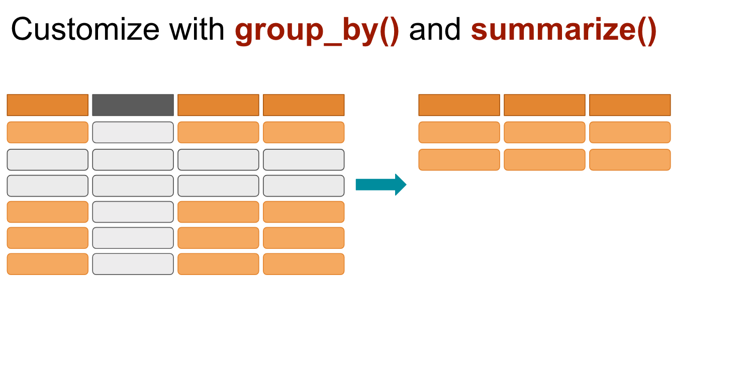
`group_by` and `summarise()`

Use when you want to aggregate your data (by groups).
Sometimes we want to calculate group statistics.

`group_by` and `summarise()`

Suppose we want to know the average population by continent.

data

data
# A tibble: 1,704 × 6
   country     continent  year lifeExp      pop gdpPercap
   <fct>       <fct>     <int>   <dbl>    <int>     <dbl>
 1 Afghanistan Asia       1952    28.8  8425333      779.
 2 Afghanistan Asia       1957    30.3  9240934      821.
 3 Afghanistan Asia       1962    32.0 10267083      853.
 4 Afghanistan Asia       1967    34.0 11537966      836.
 5 Afghanistan Asia       1972    36.1 13079460      740.
 6 Afghanistan Asia       1977    38.4 14880372      786.
 7 Afghanistan Asia       1982    39.9 12881816      978.
 8 Afghanistan Asia       1987    40.8 13867957      852.
 9 Afghanistan Asia       1992    41.7 16317921      649.
10 Afghanistan Asia       1997    41.8 22227415      635.
# ℹ 1,694 more rows

grouped_by_continent <- group_by(data, continent)
summarise(grouped_by_continent, avg_pop = mean(pop))

grouped_by_continent <- group_by(data, continent)
summarise(grouped_by_continent, avg_pop = mean(pop))
# A tibble: 5 × 2
  continent   avg_pop
  <fct>         <dbl>
1 Africa     9916003.
2 Americas  24504795.
3 Asia      77038722.
4 Europe    17169765.
5 Oceania    8874672.

`group_by` and `summarise()`

Suppose we want to know the average population by continent.

data

data
# A tibble: 1,704 × 6
   country     continent  year lifeExp      pop gdpPercap
   <fct>       <fct>     <int>   <dbl>    <int>     <dbl>
 1 Afghanistan Asia       1952    28.8  8425333      779.
 2 Afghanistan Asia       1957    30.3  9240934      821.
 3 Afghanistan Asia       1962    32.0 10267083      853.
 4 Afghanistan Asia       1967    34.0 11537966      836.
 5 Afghanistan Asia       1972    36.1 13079460      740.
 6 Afghanistan Asia       1977    38.4 14880372      786.
 7 Afghanistan Asia       1982    39.9 12881816      978.
 8 Afghanistan Asia       1987    40.8 13867957      852.
 9 Afghanistan Asia       1992    41.7 16317921      649.
10 Afghanistan Asia       1997    41.8 22227415      635.
# ℹ 1,694 more rows

grouped_by_continent <- group_by(data, continent)
summarised_data <- summarise(grouped_by_continent, avg_pop = mean(pop))
arrange(summarised_data, desc(avg_pop))

grouped_by_continent <- group_by(data, continent)
summarised_data <- summarise(grouped_by_continent, avg_pop = mean(pop))
arrange(summarised_data, desc(avg_pop))
# A tibble: 5 × 2
  continent   avg_pop
  <fct>         <dbl>
1 Asia      77038722.
2 Americas  24504795.
3 Europe    17169765.
4 Africa     9916003.
5 Oceania    8874672.

Too many codes!

It’s hard to follow!

It’s hard to keep track of the codes!

`%>%` pipe operator

The`%>%`operator

The %>% helps your write code in a way that is easier to read and understand.

grouped_by_continent <- group_by(data, continent)
summarised_data <- summarise(grouped_by_continent, avg_pop = mean(pop))
arrange(summarised_data, desc(avg_pop))

grouped_by_continent <- group_by(data, continent)
summarised_data <- summarise(grouped_by_continent, avg_pop = mean(pop))
arrange(summarised_data, desc(avg_pop))
# A tibble: 5 × 2
  continent   avg_pop
  <fct>         <dbl>
1 Asia      77038722.
2 Americas  24504795.
3 Europe    17169765.
4 Africa     9916003.
5 Oceania    8874672.

data %>% 
  group_by(continent) %>% 
  summarise(avg_pop = mean(pop)) %>% 
  arrange(desc(avg_pop))

data %>% 
  group_by(continent) %>% 
  summarise(avg_pop = mean(pop)) %>% 
  arrange(desc(avg_pop))
# A tibble: 5 × 2
  continent   avg_pop
  <fct>         <dbl>
1 Asia      77038722.
2 Americas  24504795.
3 Europe    17169765.
4 Africa     9916003.
5 Oceania    8874672.

The`%>%`operator

What is the average life expectancy of Asian countries per year?

filtered_by_asia <- filter(data, continent == "Asia")
grouped_by_country_year <- group_by(filtered_by_asia, country, year)
summarise(grouped_by_country_year, avg_lifeExp = mean(lifeExp))

filtered_by_asia <- filter(data, continent == "Asia")
grouped_by_country_year <- group_by(filtered_by_asia, country, year)
summarise(grouped_by_country_year, avg_lifeExp = mean(lifeExp))
# A tibble: 396 × 3
# Groups:   country [33]
   country      year avg_lifeExp
   <fct>       <int>       <dbl>
 1 Afghanistan  1952        28.8
 2 Afghanistan  1957        30.3
 3 Afghanistan  1962        32.0
 4 Afghanistan  1967        34.0
 5 Afghanistan  1972        36.1
 6 Afghanistan  1977        38.4
 7 Afghanistan  1982        39.9
 8 Afghanistan  1987        40.8
 9 Afghanistan  1992        41.7
10 Afghanistan  1997        41.8
# ℹ 386 more rows

data %>% 
  filter(continent == "Asia") %>% 
  group_by(country, year) %>% 
  summarise(avg_lifeExp = mean(lifeExp))

data %>% 
  filter(continent == "Asia") %>% 
  group_by(country, year) %>% 
  summarise(avg_lifeExp = mean(lifeExp))
# A tibble: 396 × 3
# Groups:   country [33]
   country      year avg_lifeExp
   <fct>       <int>       <dbl>
 1 Afghanistan  1952        28.8
 2 Afghanistan  1957        30.3
 3 Afghanistan  1962        32.0
 4 Afghanistan  1967        34.0
 5 Afghanistan  1972        36.1
 6 Afghanistan  1977        38.4
 7 Afghanistan  1982        39.9
 8 Afghanistan  1987        40.8
 9 Afghanistan  1992        41.7
10 Afghanistan  1997        41.8
# ℹ 386 more rows

The `%>%` operator

filtered_by_asia <- filter(data, continent == "Asia")
grouped_by_country <- group_by(filtered_by_asia, country)
summarised_by_country <- summarise(grouped_by_country, avg_lifeExp = mean(lifeExp))
arrange(summarised_by_country, desc(avg_lifeExp))

filtered_by_asia <- filter(data, continent == "Asia")
grouped_by_country <- group_by(filtered_by_asia, country)
summarised_by_country <- summarise(grouped_by_country, avg_lifeExp = mean(lifeExp))
arrange(summarised_by_country, desc(avg_lifeExp))
# A tibble: 33 × 2
   country          avg_lifeExp
   <fct>                  <dbl>
 1 Japan                   74.8
 2 Israel                  73.6
 3 Hong Kong, China        73.5
 4 Singapore               71.2
 5 Taiwan                  70.3
 6 Kuwait                  68.9
 7 Sri Lanka               66.5
 8 Lebanon                 65.9
 9 Bahrain                 65.6
10 Korea, Rep.             65.0
# ℹ 23 more rows

data %>% 
  filter(continent == "Asia") %>% 
  group_by(country) %>% 
  summarise(avg_lifeExp = mean(lifeExp)) %>% 
  arrange(desc(avg_lifeExp))

data %>% 
  filter(continent == "Asia") %>% 
  group_by(country) %>% 
  summarise(avg_lifeExp = mean(lifeExp)) %>% 
  arrange(desc(avg_lifeExp))
# A tibble: 33 × 2
   country          avg_lifeExp
   <fct>                  <dbl>
 1 Japan                   74.8
 2 Israel                  73.6
 3 Hong Kong, China        73.5
 4 Singapore               71.2
 5 Taiwan                  70.3
 6 Kuwait                  68.9
 7 Sri Lanka               66.5
 8 Lebanon                 65.9
 9 Bahrain                 65.6
10 Korea, Rep.             65.0
# ℹ 23 more rows

.

Overview

R Objects

R objects

R packages

Importing data

Importing data into R

SPSS, Stata & SAS using haven package

Importing data into R

Excel files using readxl package

Importing data into R

CSV files using readr package

Basic data wrangling with Tidyverse

What is tidyverse?

Data wrangling using dplyr

dplyr

select()

select()

select()

filter()

mutate()

mutate()

rename()

arrange()

group_by and summarise()

group_by and summarise()

group_by and summarise()

Too many codes!

It’s hard to follow!

It’s hard to keep track of the codes!

%>% pipe operator

The%>%operator

The%>%operator

The %>% operator

Let’s practice

Data wrangling using `dplyr`

`dplyr`

`select()`

`select()`

`select()`

`filter()`

`mutate()`

`mutate()`

`rename()`

`arrange()`

`group_by` and `summarise()`

`group_by` and `summarise()`

`group_by` and `summarise()`

`%>%` pipe operator

The`%>%`operator

The`%>%`operator

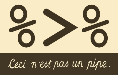
The `%>%` operator